Number extraction with Tesseract

Introduction

While comparing two different mini-maps can tell us the change in angle/heading (\(\omega\)) between them, we can determine the player’s heading (\(\theta\)) via the compass. This can be seen at the top centre of the screen (107 degrees).

_config.yml

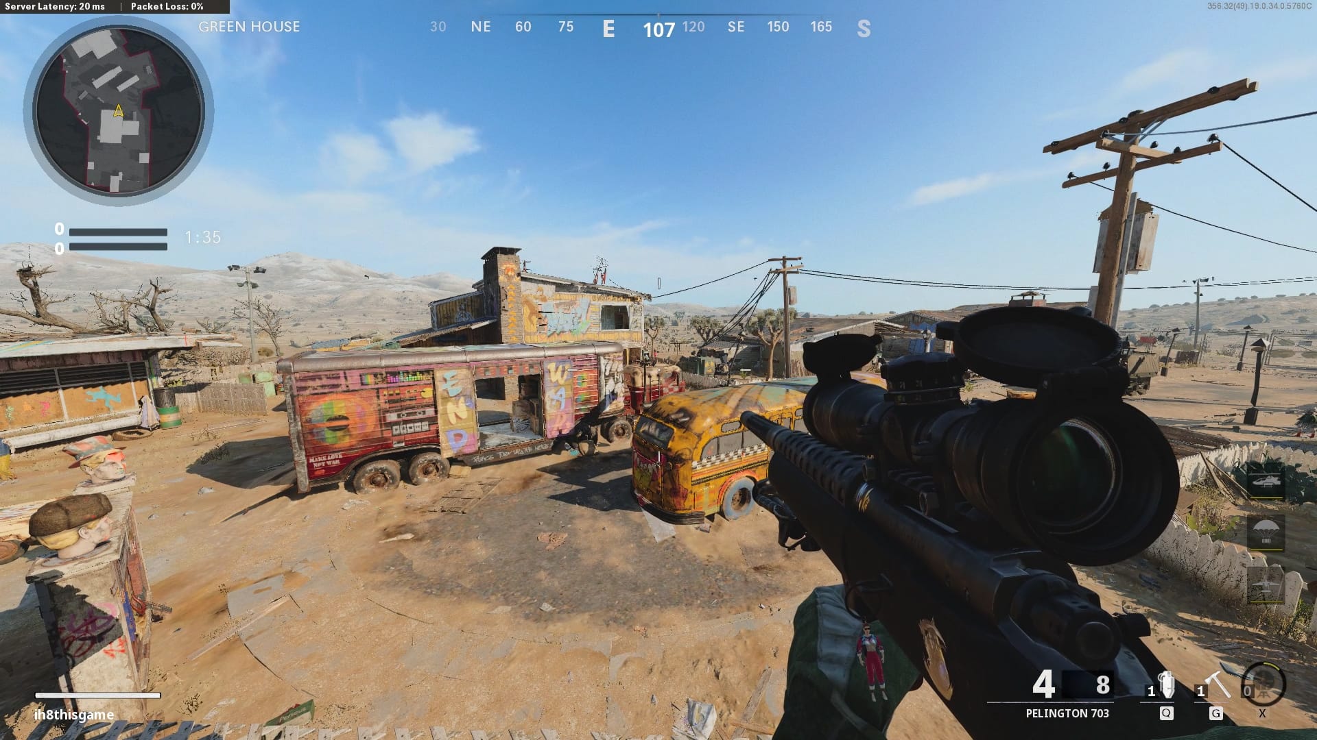
Optical Character Recognition (OCR) can read this heading, digitising the player’s current heading on a frame-by-frame basis. I’ve chosen to use Tesseract, a powerful open-source library for OCR. In Python, we can use Pytesseract, a wrapper around Tesseract.

You can find the video I’m digitising here.

import cv2
import numpy as np
import matplotlib.pyplot as plt
import seaborn as sns

import pytesseract
import re 

plt.rcParams['figure.figsize'] = [10, 10]

Pre-processing

Let’s load the first frame:

def load_frame(frame_number):
    cap.set(1, frame_number-1)
    res, frame = cap.read()
    return(frame)

Now let’s preprocess the frame by:

1. Cropping the image down so that it only contains the number.
2. Resize the image so that it’s larger.
3. Converting the image to grayscale and then inverting.

Each of these steps helps improve the accuracy of Tesseract.

def preprocess_frame(img):
    img = img[10:50,610:670,::-1]
    img = cv2.resize(img,(600,400))
    img = 255 - cv2.cvtColor(img, cv2.COLOR_BGR2GRAY)
    return(img)

Once Tesseract has processed the image, we want to extract both the angle and how confident Tesseract was in its detection from the metadata. Often when Tesseract digitises a number, it will include other characters, which we need to strip out using “re.sub(”[^0-9^]“,”“,text)”.

def extract_angle_confidence(result_dict):
    angle = np.NaN
    confidence = np.NaN
    for i in range(0,len(result_dict['text'])):
        confidence = int(result_dict['conf'][i])
        if confidence > 0:
            text = result_dict['text'][i]
            text = re.sub("[^0-9^]", "",text)
            if len(text)>0:
                angle = int(text)
                
    return(angle, confidence)            

Let’s now extract a single frame:

cap = cv2.VideoCapture('../HighRes.mp4')
img = load_frame(0,cap)
plt.imshow(img[:,:,::-1])
plt.show()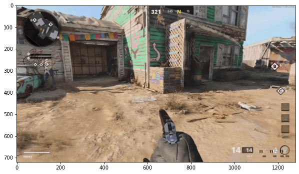

_config.yml

And after preprocessing:

img = preprocess_frame(img)
plt.imshow(img,cmap='gray')
plt.show()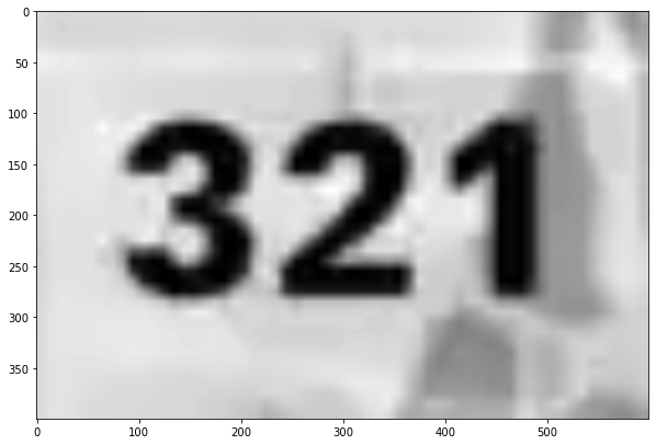

_config.yml

Processing

Now that we have preprocessed our images, it’s time to use Tesseract to digitise the text.

We have the opportunity to configure Tesseract; you can read more about the options available here.

tesseract_config = r'--oem 3 --psm 13'
result_dict = pytesseract.image_to_data(img, config = tesseract_config, output_type = pytesseract.Output.DICT)

Let’s now process the first 5,000 frames from the video:

angles = []
confidences = []
for i in range(0,5_000):
    img = load_frame(i,cap)
    img = preprocess_frame(img)

    tesseract_config = r'--oem 3 --psm 13'
    result_dict = pytesseract.image_to_data(img, config = tesseract_config, output_type = pytesseract.Output.DICT)
    
    angle, confidence = extract_angle_confidence(result_dict)
    
    angles.append(angle)
    confidences.append(confidence)

We can save both the angles and Tesseract’s level of confidence.

angles = np.array(angles)
confidences = np.array(confidences)

np.save('angles.npy',angles)
np.save('confidences.npy',confidences)

Results Analysis

---

Finally, let’s do a quick analysis of the data extracted.

By examining the histogram, we find that Tesseract often needed to be more certain about its results.

ax = sns.histplot(confidences,bins = np.arange(0,100,10))
ax.set_xlabel('Confidence (%)')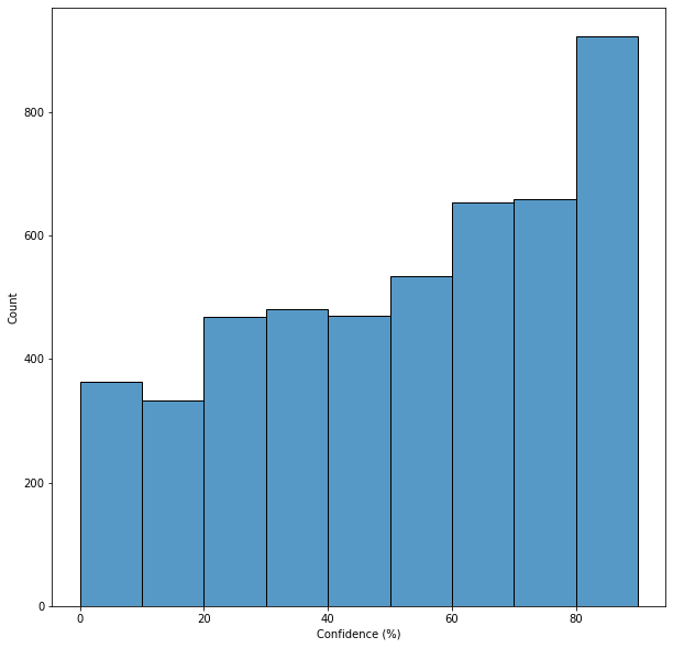

_config.yml

We can also chart the angles on a frame-by-frame basis. Note that the limits of the chart are set to the range of 0-360 (degrees).

plt.plot(angles,alpha=0.5)
plt.ylim(0,360)
plt.xlabel('Sample Number')
plt.ylabel('Angle (Degrees)')
plt.show()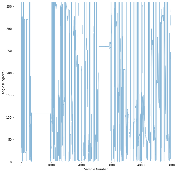

_config.yml

Using:

np.count_nonzero(~np.isnan(angles))

We find that Tesseract extracted numbers in 4,049 out of 5,000 frames.

Conclusion

Our next step is to integrate this heading data with other data sources to form a more coherent view of the player’s position and heading. We already see that our method must be robust to missing and erroneous data.