256 shades of grey

On February 22, 2000, after 11 days of measurements, the most comprehensive map ever created of the earth’s topography was complete. The space shuttle Endeavor had just completed the Shuttle Radar Topography Mission, using a specialised radar to image the earth’s surface.

The resulting Digital Elevation Map (DEM) is in the public domain and provides the measured terrain height at ~90-meter resolution. The mission mapped 99.98% of the area between 60 degrees North and 56 degrees South.

This post will examine how to process the raw DEM to be more intuitively interpreted through hill-shading, slope shading & hypsometric tinting.

Transforming the raw GeoTIFF into the final imagery product is simple. GDAL, the Geospatial Data Abstraction Library, carries out much of the grunt work.

In order, we need to:

1. Download a DEM as a GeoTIFF
2. Extract a subsection of the GeoTIFF
3. Reproject the subsection
4. Make an image with hill shading
5. Make an image by colouring the subsection according to altitude
6. Make an image by colouring the subsection according to the slope
7. Combine the three images into a final composite

DEM

Several different DEMs have been created from the data collected on the SRTM mission. I will use the CGIAR SRTM 90m Digital Elevation Database. Data is provided in 5x5 degree tiles, with each degree of latitude equal to approximately 111 km.

Our first task is to acquire a tile. Tiles can be downloaded from here using wget.

import os
import math
from PIL import Image, ImageChops, ImageEnhance
from matplotlib import cm

def downloadDEMFromCGIAR(lat,lon):
    ''' Download a DEM from CGIAR FTP repository '''
    fileName = lonLatToFileName(lon,lat)+'.zip'

    ''' Check to see if we have already downloaded the file '''
    if fileName not in os.listdir('.'):
        os.system('''wget --user=data_public --password='GDdci' http://data.cgiar-csi.org/srtm/tiles/GeoTIFF/'''+fileName)
    os.system('unzip '+fileName)

def lonLatToFileName(lon,lat):
    ''' Compute the input file name '''
    tileX = int(math.ceil((lon+180)/5.0))
    tileY = -1*int(math.ceil((lat-65)/5.0))
    inputFileName = 'srtm_'+str(tileX).zfill(2)+'_'+str(tileY).zfill(2)
    return(inputFileName)

lon,lat = -123,49
inputFileName = lonLatToFileName(lon,lat)
downloadDEMFromCGIAR(lat,lon)

Slicing

The area I have selected covers Washington State and British Columbia, with file name srtm_12_03.tif.

Let’s use GDAL to extract a subsection of the tile. The subsection covers Vancouver Island and the Pacific Ranges, stretching from 125ºW - 122ºW & 48ºN - 50ºN. Using gdalwarp:

!! gdalwarp -q -te -125 48 -122 50 -srcnodata -32768 -dstnodata 0 srtm_12_03.tif subset.tif

Our next step is to transform the subsection of the tile to a different projection. The points in the subsection are located on a grid 1/1200th of a degree apart. A separate scale exists between the latitude & longitude axis and a longitude scale that depends on the latitude. While degrees of latitude are always ~110 km in size, resulting in ~92.5M resolution, degrees of longitude decrease from ~111 km at the equator to 0 km at the poles.

A solution is to project that points to have a consistent and equal scale in the X/Y plane. One choice is to use a family of projections called Universal Transverse Mercator. Each UTM projection can map points from longitude & latitude to X & Y coordinates in meters. The UTM projection is helpful because it locally preserves both shapes and distances over distances of up to several hundred kilometres.

The tradeoff is that several different UTM projections are required for different points on earth, 120 to be precise. Fortunately, working out the required projection based on the longitude and latitude is relatively trivial. Almost every conceivable projection has been assigned a code by the European Petroleum Survey Group (EPSG). You can use this EPSG code to specify the projection being used unambiguously. With UTM, each code starts with either 327 or 326, depending on the hemisphere of the projection.

utmZone = int((math.floor((lon + 180)/6) % 60) + 1)

''' Check to see if the file is in the northern or southern hemisphere '''
if lat<0:
    EPSGCode = 'EPSG:327'+str(utmZone)
else:
    EPSGCode = 'EPSG:326'+str(utmZone)

Once we have identified the correct EPSG code to use, warping the subset to a new projection is relatively straightforward.

In the following system call to gdalwarp, t_srs denotes the target projection, and tr specifies the resolution in the X and Y plane. The Y resolution is negative because the GDAL file uses a (row, column) coordinate system.

In this coordinate system, the origin is in the top left-hand corner of the file. The row value increases as you move down the file, like an excel spreadsheet; however, the UTM Y coordinate decreases. This results in a negative sign in the resolution.

os.system('gdalwarp -q -t_srs '+EPSGCode+' -tr 100 -100 -r cubic subset.tif warped.tif')

Hillshading

At this point, we can begin to visualise the DEM. One highly effective method is hill-shading, which models how the surface of the DEM would be illuminated by light projected onto it. Shading of the slopes allows the DEM to be more intuitively interpreted than just colouring by height alone.

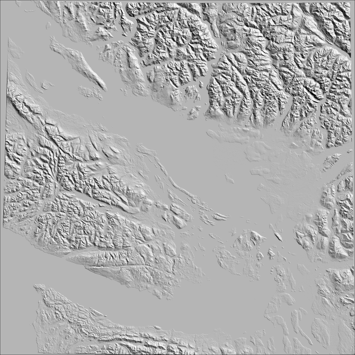
!! gdaldem hillshade -q -az 45 -alt 45 warped.tif hillshade.tif

Hypsometric Tinting

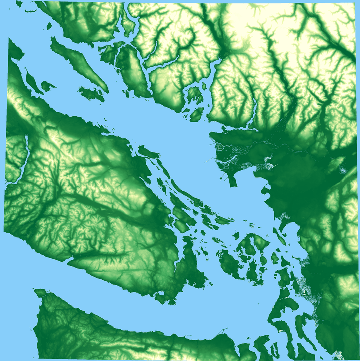
Hillshading can also be combined with height information to aid the interpretation of the topography. The process is simple, with GDAL mapping colours to cell heights using a provided colour scheme. The technical name for colouring a DEM based on height is hypsometric tinting.

def createColorMapLUT(minHeight,maxHeight,cmap = cm.YlGn_r,numSteps=256):
    '''
    Create a colourmap for visualisation
    '''
    f =open('color_relief.txt','w')
    f.write('-0.1,135,206,250 \n')
    f.write('0.1,135,206,250 \n')
    
    for i in range(0,numSteps):
        r,g,b,a= cmap(i/float(numSteps))
        height = minHeight + (maxHeight-minHeight)*(i/numSteps)
        f.write(str(height)+','+str(int(255*r))+','+str(int(255*g))+','+str(int(255*b))+'\n')
    f.write(str(-1)+','+str(int(255*r))+','+str(int(255*g))+','+str(int(255*b))+'\n')
    

createColorMapLUT(minHeight=10,maxHeight=2658)

!! gdaldem color-relief -q warped.tif color_relief.txt color_relief.tif

Slope Shading

Another technique for visualising terrain is slope shading. While hypsometric tinting assigns colours to cells based on elevation, slope shading assigns colours to pixels based on the slope (0º to 90º). In this case, white (255,255,255) is assigned to slopes of 0º and black (0,0,0) is assigned to slopes of 90º, with varying shades of grey for slopes in-between.

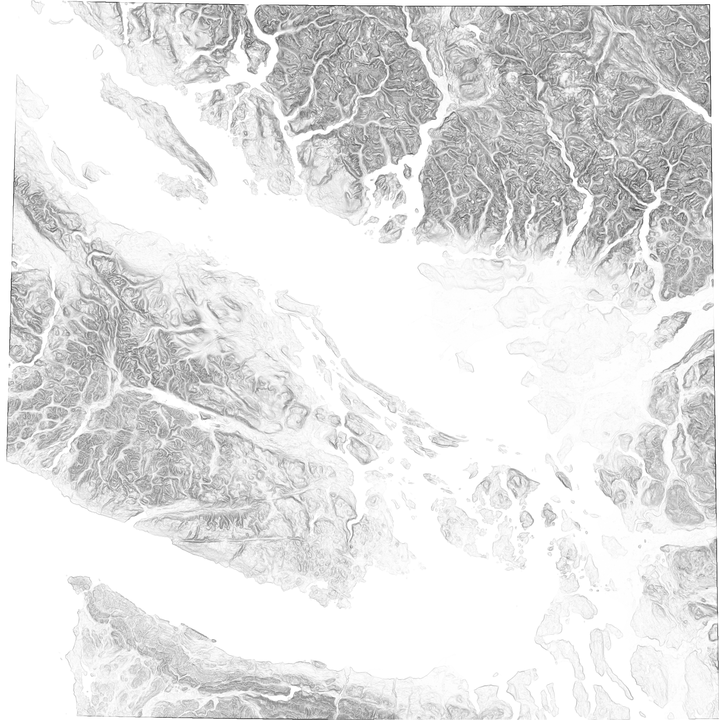
This colour scheme is encoded in a txt file for gdaldem as follows:

f = open('color_slope.txt','w')
f.write('0 255 255 255\n')
f.write('90 0 0 0\n')
f.close()

The computation of the slope shaded dem takes place over two steps.

1. The slope of each cell is computed.
2. Each cell is assigned a shade of grey depending on the slope.

!! gdaldem slope -q warped.tif slope.tif
!! gdaldem color-relief -q slope.tif color_slope.txt slopeshade.tif

Layer Merging

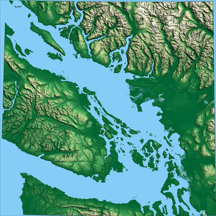
The final step in producing the final product is to merge the three different created images. The Python Image Library (PIL) is a quick and dirty way to accomplish this task, combining the three layers using pixel-by-pixel multiplication.

One crucial detail to note is that the pixel-by-pixel multiplication occurs in the RGB space. Theoretically, each pixel should be first transformed to the Hue, Saturation, Value (HSV) colour space. The value is then multiplied by the hill-shade and slope-shade values before being transformed into the RGB colour space. However, the RGB space multiplication is a very reasonable approximation in practical terms.

In one final tweak, the brightness of the output image is increased by 40% to offset the average reduction in brightness caused by multiplying the layers together.

''' Merge components using Python Image Lib '''
slopeshade = Image.open("slopeshade.tif").convert('L')
hillshade = Image.open("hillshade.tif")
colorRelief = Image.open("color_relief.tif")

# Let's fill in any gaps in the hill shading
ref = Image.new('L', slopeshade.size,180)
hillshade = ImageChops.lighter(hillshade,ref)

shading = ImageChops.multiply(slopeshade, hillshade).convert('RGB')
merged = ImageChops.multiply(shading,colorRelief)

''' Adjust the brightness to take into account the reduction caused by hill shading.''
enhancer = ImageEnhance.Brightness(merged)
img_enhanced = enhancer.enhance(1.4)
img_enhanced.save('Merged.png')

Further reading

I found the following sources to be invaluable in compiling this post:

• Creating colour relief and slope shading
• A workflow for creating beautiful relief-shaded DEMs using gdal
• Shaded relief map in python
• Stamen Design