Kalman Filters are magic. While they take 5 minutes to explain at a basic level, you can work with them for a career and always be learning more. There is something philosophically satisfying about how they innately combine what we already believe and what we perceive to come to a new belief about the world.

While this sounds abstract, Kalman Filters provide a concrete mathematical formulation for fusing data from different sources and physical models to provide (potentially) optimum estimates of the state of a system.

For less philosophy and more maths, I strongly recommend stopping at this point and giving this excellent post a read. Afterwards, let’s concretely talk about Kalman filters,

Creating a Kalman Filter in 7 easy steps:

One of the challenges with Kalman filters is that it’s easy to be initially overwhelmed by the mathematical background and lose sight of their implementation in practice. In reality, it’s possible to break the implementation down into a series of discrete steps, which come together to describe the filter fully.

FilterPy is a great Python library for creating Kalman filters and has an accompanying book that takes a deep dive into the mathematical theory of Kalman filters. Let’s initially discuss the general process for defining a Kalman filter before applying it to practical application.

x: Our filter state estimate, IE, what we want to estimate. If we’re going to track an object moving in a video, this could be its pixel coordinates and its velocity in pixels per second. [x,y,vx,vy]
P: The covariance matrix. It encodes how sure the filter is about its estimates and evolves over time. In the object tracking example, how “confident” the filter is about the position of an object and its velocity. As the filter receives more measurements, the values in the covariance matrix are “washed out”, so the filter tends to be insensitive to the values used.
Q: The process uncertainty. How significant is the error associated with the system doing something unexpected between measurements? This is the hardest to set, as it requires careful thought about the process. For example, if we are tracking the position and velocity of an object once a second, we would have more uncertainty if we were tracking the position of a fruit fly than an oil tanker.
R: How uncertain each of our measurements is. This can be determined either through reading sensor datasheets or educated guesses.
H: How each measurement is related to the internal state of our system, in addition to scaling measurements. If we have a GPS receiver, it tells us about our position, while an accelerometer tells us about our acceleration.
F: The state transition matrix. How the system evolves over time. IE, if we know the position and velocity of an object, then in the absence of any error or external influence, we can predict its next position from its current position and velocity.
B: The control matrix. This matrix allows us to tell the filter how we expect any inputs we provide (u) to update the system’s state. In many cases, the control matrix is not required, especially when we take measurements of a system we don’t control.

At this point, it’s worthwhile considering how these matrices are related. Tim Babb of Bzarg has a fantastic diagram that sets out how information flows through the filters mentioned above. If you haven’t already, I strongly recommend you read his post on how Kalman filters work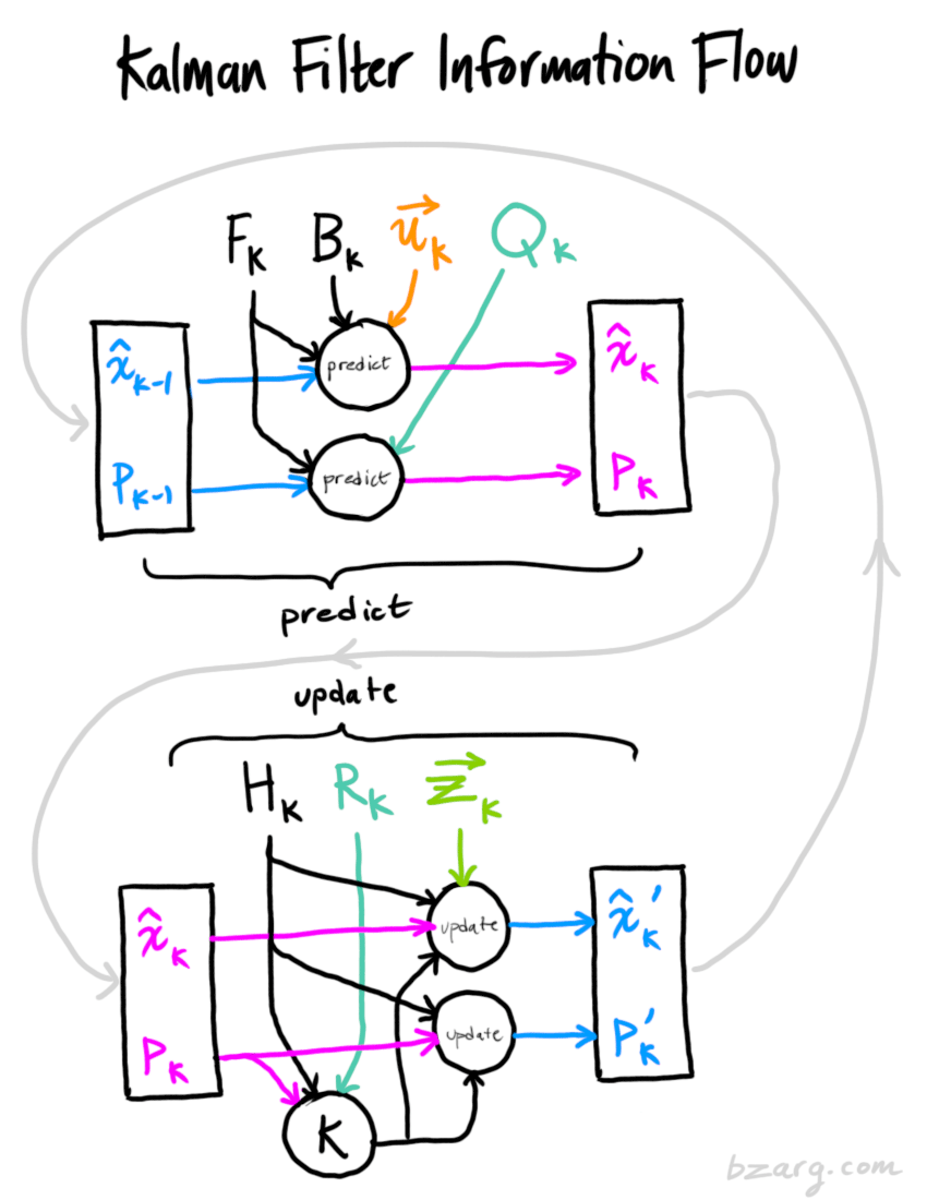

Looking at the relationships between all of the matrices,

x and P are the filter outputs; they tell what the filter believes the system’s state to be.
H, F and B are matrices that control the filter’s operation.
Qand R are closely related because they denote uncertainty in the process and the measurements.
z and u denote inputs to the filter. If we don’t control the system, then u is not required.

A real-world example:

In computer vision, object tracking associates different detections of an object from different images/frames into a single “track”. Many algorithms have been developed for this task Simple Online and Realtime Tracking is particularly elegant. Let’s look at a real-world example. In summary, SORT creates a Kalman filter for each object it wants to track and then predicts the location and size of each object in each frame using the filter.

Alex Bewley, one of the creators of SORT, has developed a fantastic implementation of SORT, which uses Filterpy.

Let’s take a look at his implementation through the lens of what I’ve discussed above:

Quickly defining some nomenclature,

u and v are the x and y pixel coordinates of the centre of the bounding box around an object being tracked.
s and r are the scale and aspect ratio of the bounding box surrounding the object.
\(\dot u, \dot v\) are the x and y velocity of the bounding box.
\(\dot s\) is the rate at which the bounding box’s scale changes.

kf = KalmanFilter(dim_x=7, dim_z=4)

Our internal state is seven-dimensional: \([u, v, s, r, \dot u, \dot v , \dot s]\)

While our input vector is four-dimensional: \([u, v, s, r]\)

kf.F = np.array([[1,0,0,0,1,0,0],
                 [0,1,0,0,0,1,0],
                 [0,0,1,0,0,0,1],
                 [0,0,0,1,0,0,0], 
                 [0,0,0,0,1,0,0],
                 [0,0,0,0,0,1,0],
                 [0,0,0,0,0,0,1]])

The state transition matrix tells us that at each timestep, we update our state as follows:

\[u = u + \dot u\]

\[v = v + \dot v\]

\[s = s + \dot s\]

kf.H = np.array([[1,0,0,0,0,0,0],
                 [0,1,0,0,0,0,0],
                 [0,0,1,0,0,0,0],
                 [0,0,0,1,0,0,0]])

The sensor matrix tells us that we directly measure \([u, v, s, r]\).

kf.R = np.array([[ 1,  0,  0,  0],
                 [ 0,  1,  0,  0,],
                 [ 0,  0, 10,  0,],
                 [ 0,  0,  0, 10,]])

The sensor noise matrix tells us that we can measure \(u\) and \(v\) with a much higher certainty than \(s\) and \(r\).

kf.P = np.array([[   10,    0,     0,     0,     0,     0,     0],
                 [    0,   10,     0,     0,     0,     0,     0],
                 [    0,    0,    10,     0,     0,     0,     0],
                 [    0,    0,     0,    10,     0,     0,     0],
                 [    0,    0,     0,     0, 10000,     0,     0],
                 [    0,    0,     0,     0,     0, 10000,     0],
                 [    0,    0,     0,     0,     0,     0, 10000]])

The covariance matrix tells us that the filter should have a very high initial uncertainty for each velocity component.

kf.Q = np.array([[1.e+00, 0.e+00, 0.e+00, 0.e+00, 0.e+00, 0.e+00, 0.e+00]
                 [0.e+00, 1.e+00, 0.e+00, 0.e+00, 0.e+00, 0.e+00, 0.e+00]
                 [0.e+00, 0.e+00, 1.e+00, 0.e+00, 0.e+00, 0.e+00, 0.e+00]
                 [0.e+00, 0.e+00, 0.e+00, 1.e+00, 0.e+00, 0.e+00, 0.e+00]
                 [0.e+00, 0.e+00, 0.e+00, 0.e+00, 1.e-02, 0.e+00, 0.e+00]
                 [0.e+00, 0.e+00, 0.e+00, 0.e+00, 0.e+00, 1.e-02, 0.e+00]
                 [0.e+00, 0.e+00, 0.e+00, 0.e+00, 0.e+00, 0.e+00, 1.e-04]])

The Process uncertainty matrix tells us how much “uncertainty” is in each system’s behaviour component.

Filterpy has a function that can be very useful for generating Q.

filterpy.common.Q_discrete_white_noise

Creating a Kalman Filter in 7 easy steps:

A real-world example:

Further reading