import numpy as np
import matplotlib.pyplot as plt
plt.rcParams['figure.figsize'] = [15, 15]

# E: the data
y = np.array([52, 145, 84, 161, 85, 152,
       47, 109, 16, 16, 106, 101,
       64, 73, 57, 83, 88, 135,
       119,120,121, 122, 42, 8, 8, 104, 112,
       89, 82, 74, 114, 22, 12,
       21, 21, 67, 71, 93, 94,
       75, 7, 97, 117, 62, 87,
       55, 11, 38, 80, 72, 43,
       50, 86, 31, 108, 24, 24,
       95, 132, 103, 77, 113, 78,
       32, 32, 41, 18, 14, 14,
       79, 66, 65, 81, 105, 53,
       98, 98, 111, 163, 102,
       34, 107, 59, 10, 61, 29,
       46, 4, 4, 30, 37, 76, 44,
       54, 90, 48, 13, 118, 100,
       56, 63, 51, 68, 19, 25,
       23, 13, 110, 26, 17, 33,
       20, 124, 146, 147, 131, 91, 116,
       58, 99, 160, 20, 20, 9,
        6, 115, 69, 136, 92, 128,
       60, 15, 27, 27, 151, 138,
       130, 125, 162, 159, 3, 137,
       155, 144, 126, 158, 149,
150])An Introduction to PyMC3
In the Last post, I took a first-principles approach to solve a Bayesian analysis problem computationally. In practice, problems can be far more complex. Fortunately, sophisticated software libraries already exist. We can leverage that to solve equally tricky problems. While several options are available, my current favourite is PyMC3.
If you want to be inspired by what’s possible, I strongly suggest checking out the fantastic set of examples on the PyMC3 site.
Putting it into practice
Let’s start as we did last time by taking a sample of the first ten elements from the blacklist.
y_sample = y[0:10]
plt.stem(np.sort(y_sample), use_line_collection=True)
plt.show()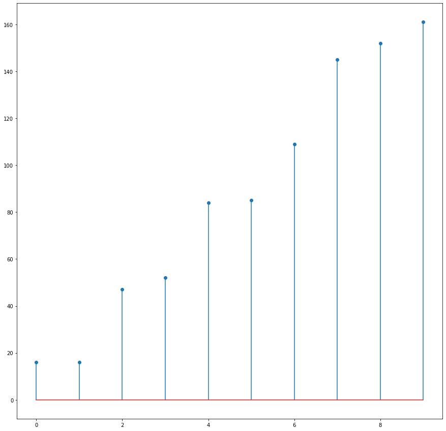
Now, this is when things start getting interesting. Firstly I will lay out all the code we need to solve this problem, all seven lines.
import pymc3 as pm

model = pm.Model()
with model:
    # prior - P(N): N ~ uniform(max(y), 500)
    N = pm.DiscreteUniform("N", lower=y.max(), upper=500)

    # likelihood - P(D|N): y ~ uniform(0, N)
    y_obs = pm.DiscreteUniform("y_obs", lower=0, upper=N, observed=y)

    trace = pm.sample(10_000, start={"N": y.max()})

pm.plots.plot_posterior(trace)
Multiprocess sampling (2 chains in 2 jobs)
Metropolis: [N]
Sampling 2 chains, 0 divergences: 100%|██████████| 21000/21000 [00:05<00:00, 4179.11draws/s]
The number of effective samples is smaller than 10% for some parameters.array([<AxesSubplot:title={'center':'N'}>], dtype=object)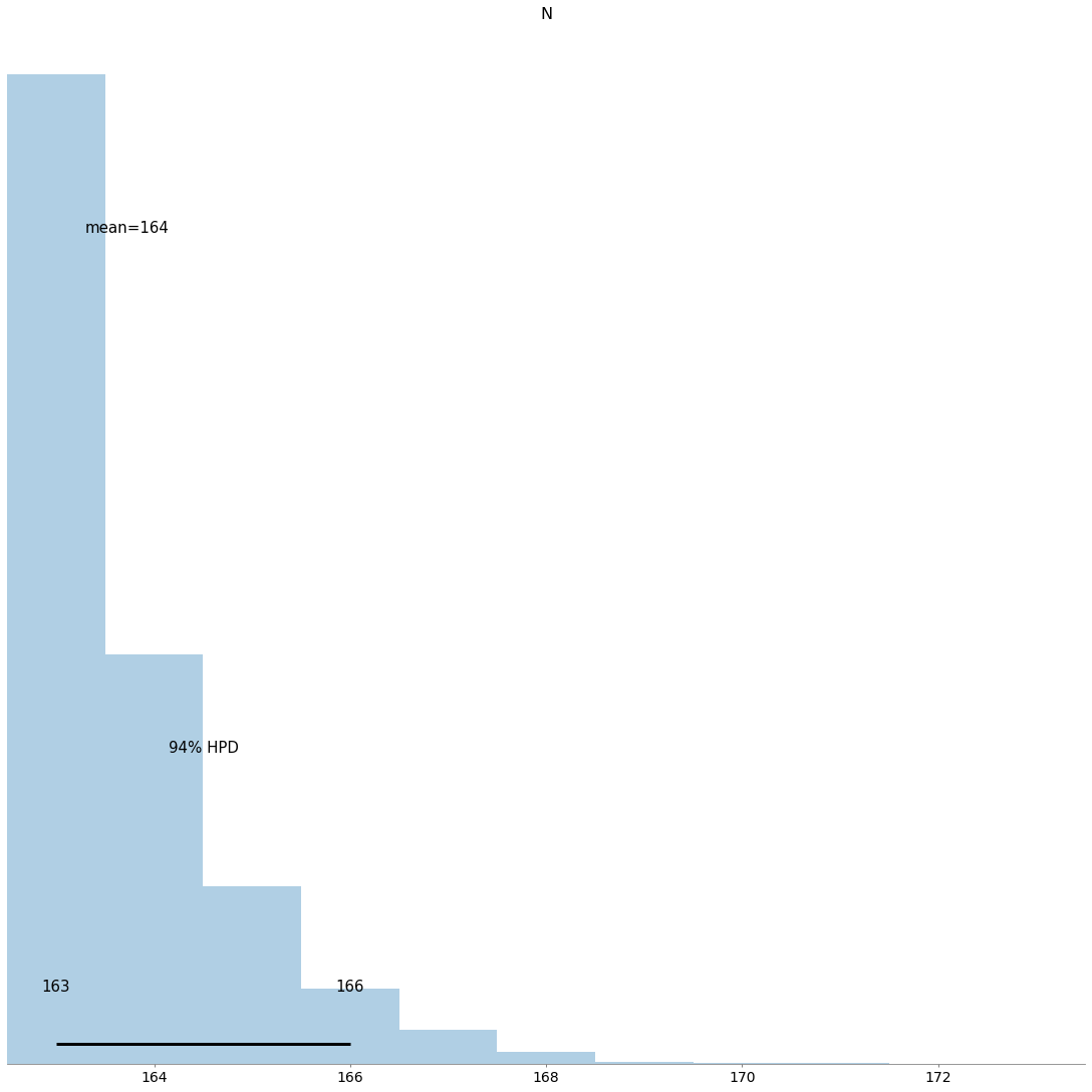
Ok, we are 94% confident the answer (the length of the Blacklist) is in the range of 163 to 166.
Line by Line.
Let’s step through now, line by line, to understand what’s going on.
- Import PyMC3.
import pymc3 as pm- Create a PyMC3 model.
model = pm.Model()- Create a context manager so that that magic can happen behind the scenes
with model:- Create a distribution for \(N\), our prior belief of the length of the Blacklist (\(P(H)\)). In layperson’s terms, $ N $ is equally likely to be any integer between the highest index we observe in our sample of data, 500. The number 500 is arbitrary; ultimately, the data we observe will “wash out” any assumptions we have made.
N = pm.DiscreteUniform("N", lower=y.max(), upper=500)- Create our likelihood function, \(P(E|H)\). Given the data we have observed, how likely is any value of N? Again, we are using a discrete uniform distribution to model the probability of seeing any observed data point.
y_obs = pm.DiscreteUniform("y_obs", lower=0, upper=N, observed=y)- Sample the model. We are computationally finding \(P(H|E)\). This is where the real magic occurs. In this case, we generate 10,000 samples and store them in ‘trace’.
trace = pm.sample(10_000, start={"N": y.max()}) - Plot the distribution of the parameters. This is our posterior, (\(P(H|E)\)).
pm.plots.plot_posterior(trace)Conclusion
In conclusion, PyMC3 can quickly and efficiently conduct Bayesian analysis. I hope to do more examples in future posts, looking at other ‘real world’ problems.